⚗️ Hamilton Zoo Advanced Analytics 📊 Tātari Arō Kōpere Kirikiriroa
🎯 Advanced Mathematical Investigation | Rangahau Pāngarau Arā
Welcome to professional-level spatial analysis! You'll use advanced coordinate geometry and mathematical modelling to solve complex zoo management challenges.
📊 Advanced Mathematical Concepts:
🔢 Core Mathematics:
- Four-quadrant coordinate system
- Distance & midpoint formulas
- Linear equations & gradients
- Geometric transformations
- Optimisation techniques
🔬 Applied Analysis:
- Mathematical modelling
- Data interpretation
- Constraint optimisation
- Statistical relationships
- Professional problem-solving
Extended coordinate plane: Scale 1 unit = 1 grid square = 80 m | Origin at zoo geometric centre
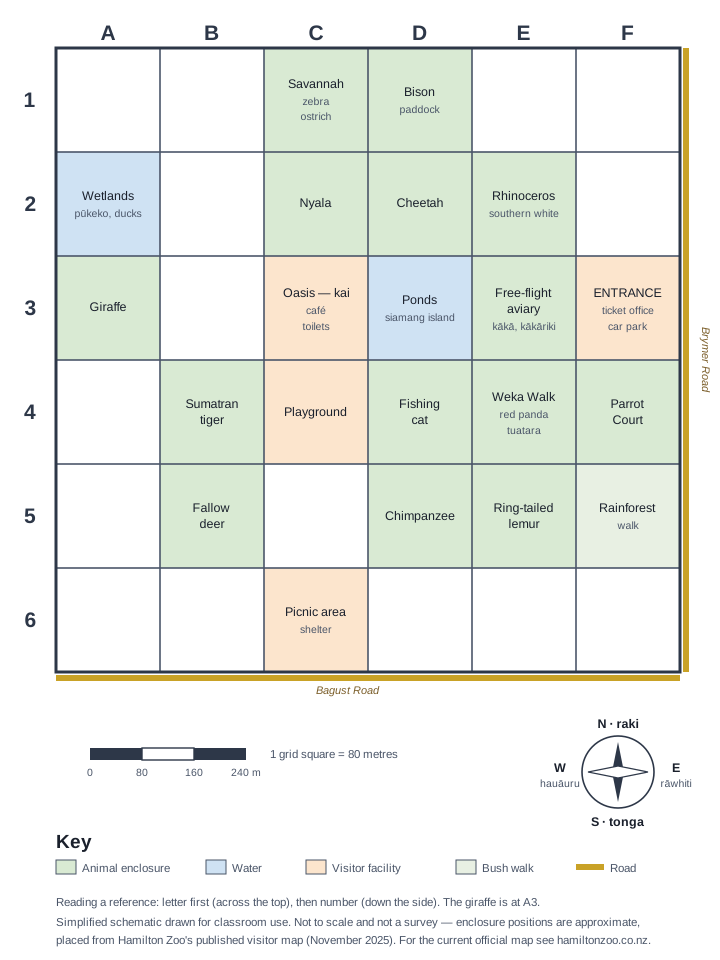
Investigation 1: Four-Quadrant Coordinate Mapping
Research Question: How can we use an extended coordinate system to optimise zoo layout and operations across all quadrants?
📍 Extended Coordinate System Setup:
Origin (0, 0): Zoo geometric centre
Quadrant I (+, +): Main exhibits and visitor areas
Quadrant II (-, +): Research facilities and breeding programs
Quadrant III (-, -): Infrastructure (parking, maintenance, storage)
Quadrant IV (+, -): Future expansion zone and conservation areas
Scale Factor: 1 coordinate unit = 1 grid square = 80 metres
Two layers, stated plainly: the Hamilton Zoo map you already know answers where — letter-number squares (A–F across, 1–6 down). The quadrant model on this page answers a different question — what kind of land use — so it divides the site by operations, not by map letters: main exhibits and visitor areas in Quadrant I, research and breeding in II, infrastructure in III, future expansion in IV. To place a facility in the model, read its map square for direction and rough distance from the site centre, then choose a signed coordinate pair that satisfies its zone's sign conditions — a modelling decision you state and defend, like a surveyor choosing axes. Converting a map position such as B5 into a defended (x, y) pair is a skill the investigations below will repeatedly ask of you.
The sign conditions built into each answer box are the point, not a hint: a coordinate pair only counts if it satisfies its zone's quadrant signs. Choose values, then check them against the conditions.
| Facility | Quadrant | x-coordinate | y-coordinate | Coordinate Pair | Real Distance from Origin (m) |
|---|---|---|---|---|---|
| 🚗 Main Car Park | III | ( , ) | |||
| 🦒 Giraffe Exhibit | I | ( , ) | |||
| 🔬 Research Centre | II | ( , ) | |||
| 🌱 Future Conservation Zone | IV | ( , ) |
Investigation 2: Linear Modelling & Gradient Analysis
Research Question: How can linear relationships model visitor flow patterns and optimise pathway efficiency?
📊 Visitor Flow Analysis
Zoo data shows visitor movement follows predictable linear patterns between major attractions.
Task 1: Pathway Gradient Calculation
Calculate the gradient of the main pathway from Car Park to Giraffe Exhibit:
Car Park: ( , )
Giraffe Exhibit: ( , )
Interpretation: A gradient of means for every units horizontally, the path rises units vertically.
Task 2: Linear Equation Modelling
Develop a linear equation for the main visitor pathway using point-slope form:
y - y₁ = m(x - x₁)
Using Car Park as reference point:
y - ( ) = (x - ( ))
Investigation 3: Geometric Transformations
Research Question: How can coordinate transformations optimise zoo exhibit layouts for seasonal changes and special events?
🔄 Transformation Matrices
Apply transformation matrices to relocate the temporary petting zoo exhibit:
Original Petting Zoo Vertices:
A(2, 1), B(4, 1), C(4, 3), D(2, 3)
Translation Vector:
Move 3 units left, 2 units down
[ ]
Rotation Matrix (90°):
Rotate 90° counterclockwise about origin
[ ]
Scaling Matrix:
Scale by factor of 1.5
[ ]
Composite Transformation: T ∘ R ∘ S
Calculate the final position of vertex A(2, 1) after all transformations:
Step 1 - Scale: S × [2, 1]ᵀ = [ , ]ᵀ
Step 2 - Rotate: R × result = [ , ]ᵀ
Step 3 - Translate: T + result = [ , ]ᵀ
Investigation 4: Optimisation & Constraint Analysis
Research Question: Given multiple constraints, what is the optimal location for a new educational centre?
🎯 Multi-Constraint Optimisation Problem
Requirements for New Educational Centre:
- Must be within 5 coordinate units (400 m) of the main visitor pathway
- Cannot be more than 7.5 coordinate units (600 m) from any existing major exhibit
- Must maintain a minimum 3-coordinate-unit (240 m) buffer from animal enclosures
- Should minimise total visitor walking distance
- Must be in Quadrant I for accessibility
Mathematical Constraint Modelling:
Constraint 1: Distance from pathway y = mx + c ≤ 5 units (400m)
Point-to-line distance: d = |ax + by + c|/√(a² + b²)
Constraint 2: Maximum distance from exhibits
∀ exhibit E: √[(x - xₑ)² + (y - yₑ)²] ≤ 7.5 units (600m)
Constraint 3: Minimum buffer from enclosures
∀ enclosure F: √[(x - xf)² + (y - yf)²] ≥ 3 units (240m)
Objective Function: Minimise Σ dᵢ where dᵢ = distance to visitor attraction i
Proposed Solution:
Educational Centre Coordinates: ( , )
Constraint Verification:
| Constraint | Required | Calculated Value | Satisfied? ✓/✗ |
|---|---|---|---|
| Distance from pathway | ≤ 5.0 units | units | |
| Max distance to exhibits | ≤ 7.5 units | units | |
| Min buffer from animals | ≥ 3.0 units | units |
Total visitor walking distance: units = metres
Investigation 5: Statistical Modelling & Prediction
Research Question: How can coordinate-based analysis predict visitor patterns and optimise resource allocation?
📈 Advanced Statistical Analysis
Work from the practice dataset below — ten sampled days of peak-hour visitor centroids on the signed coordinate system. It is an illustrative practice set for computation, not real Hamilton Zoo data; treat any conclusion as about the dataset, and say so in your write-up. Compute the mean centroid and the spread, then analyse spatial patterns:
| Day | Visitors | Centroid x̄ | Centroid ȳ |
|---|---|---|---|
| 1 | 1,840 | 0.8 | 0.5 |
| 2 | 2,310 | 1.2 | 0.9 |
| 3 | 960 | −0.6 | −0.4 |
| 4 | 1,450 | 0.2 | 0.1 |
| 5 | 2,750 | 1.6 | 1.1 |
| 6 | 1,120 | −0.9 | 0.3 |
| 7 | 1,980 | 0.5 | −0.7 |
| 8 | 830 | −1.4 | −1.0 |
| 9 | 2,200 | 1.0 | 0.6 |
| 10 | 1,560 | 0.1 | −0.2 |
Heat Map Analysis
Visitor density function: ρ(x,y) = Ae^(-((x-μₓ)² + (y-μᵧ)²)/(2σ²))
Where μₓ, μᵧ are mean coordinates and σ is standard deviation
Peak visitor coordinates: μ = ( , )
Spread parameter: σ = units
Maximum density: A = visitors/unit²
Correlation Analysis
Pearson correlation coefficient between daily visitors and centroid x̄:
r = Σ[(nᵢ - n̄)(xᵢ - x̄)] / √[Σ(nᵢ - n̄)² × Σ(xᵢ - x̄)²]
Calculated correlation: r =
Interpretation:
Predictive Modelling
Linear regression for visitor numbers based on coordinates:
V(x,y) = β₀ + β₁x + β₂y + β₃xy + ε
Regression coefficients:
β₀ (intercept) =
β₁ (x-coefficient) =
β₂ (y-coefficient) =
β₃ (interaction) =
R² value:
Prediction for coordinates (2.5, 1.8): visitors/hour
🎉 Advanced Mathematics Mastery Complete! | Kua Oti te Angitū Arā!
Outstanding! You've worked through coordinate geometry and mathematical modelling that stretches well past the Years 9-10 curriculum.
✅ Mathematical Skills Mastered:
- 🎯 Four-quadrant coordinate systems
- 📐 Advanced distance & gradient formulas
- 🔄 Matrix transformations
- ⚗️ Constraint optimisation
- 📊 Statistical coordinate analysis
- 🧮 Linear regression modelling
🚀 Career Pathways Unlocked:
- 🏗️ Engineering & Architecture
- 💻 Computer Science & Gaming
- 📡 Geospatial Technology (GIS)
- 📊 Data Science & Analytics
- 🛰️ Aerospace Engineering
- 🔬 Research & Development
📚 Where this maths goes next:
- 🔢 Calculus & Advanced Mathematics
- 📊 Statistics & Probability
- 🎯 Linear Algebra
- ⚗️ Operations Research
- 💻 Computational Mathematics
- 🌍 Applied Mathematics
🎯 Teacher Notes | Ngā Kōrero Kaiako
📚 NZ Curriculum Phase 4 Alignment:
📐 Geometry & Measurement:
- Use four-quadrant coordinate systems fluently
- Apply distance, midpoint, and gradient formulas
- Understand and perform geometric transformations
- Use coordinate geometry to solve optimisation problems
- Connect geometric and algebraic representations
🔢 Algebra:
- Form and solve linear equations in context
- Use algebraic methods for constraint problems
- Apply function notation and transformations
- Model relationships using coordinate geometry
📊 Statistics:
- Use statistical methods to analyse spatial data
- Apply correlation and regression in coordinates
- Interpret statistical measures in context
- Make predictions using mathematical models
🔬 Mathematical Practices:
- Develop mathematical arguments and proofs
- Use mathematical modelling to solve problems
- Connect mathematics to other disciplines
- Communicate mathematical ideas professionally
🌿 Cultural & Career Integration:
- Tātari Arā: Advanced analysis connecting to Māori mathematical thinking
- Rangahau: Research methodologies reflecting indigenous inquiry practices
- STEM Pathways: Clear connections to tertiary study and career options
- Real-world Impact: Authentic applications in conservation and environmental management
Kaiako Planning Snapshot
Ngā Whāinga Akoranga — Learning Intentions
- Use four-quadrant coordinates, distance, midpoint, and gradient formulas to analyse Hamilton Zoo spaces with increasing precision.
- Interpret mathematical models that describe visitor movement, pathway efficiency, and exhibit layout decisions.
- Apply transformations, constraints, and statistical reasoning to justify design choices in a real-world conservation setting.
Paearu Angitu — Success Criteria
- I can calculate and interpret coordinates, gradients, and distances accurately in context.
- I can explain how a mathematical model helps solve a zoo planning or visitor-flow problem.
- I can compare possible solutions and justify which one best meets the constraints of the task.
Teacher Planning Snapshot
- Year level: Years 9-10 | Duration: Phase 4 extension sequence in advanced coordinate geometry and analytics.
- Teaching focus: Keep students moving between map, formula, and interpretation. The mathematics matters most when they can explain what a coordinate decision means for visitors, animals, staff, and conservation planning.
- Entry support: Start with a shared worked example for one zoo location pair, then provide scaffolded coordinate grids, labelled quadrants, and partially completed formula substitutions before students attempt independent modelling.
- On-level: Most learners can calculate gradients, distances, and midpoints accurately, then use those results to comment on path efficiency, exhibit placement, and design constraints.
- Extension: Ask students to create and test their own optimisation rule or predictive model for a new zoo facility, including a written justification of assumptions, limitations, and possible improvements.
Curriculum alignment
- Te Mātaiaho | Mathematics and Statistics, Phase 4 (Years 9–10): investigating and modelling in context — this unit teaches extended coordinate systems, transformation geometry, distance and constraint reasoning, linear models and their limits, and statistical prediction, under the anchor statement in the sidebar.
- NZC 2007 Mathematics, Level 5: geometry — using coordinates and the Cartesian plane; transformations — describing and performing rotations and reflections; statistics — planning and conducting investigations using data.
🔗 Unit Progression & Next Steps
Six lessons that move from building a shared coordinate model to defending a proposal somebody else can audit. Each step adds one kind of evidence — position, then distance, then transformation, then a model and its limits, then the constraints that rule options out — so the final proposal is argued from accumulated working rather than asserted at the end.
The lesson files live in the companion unit Hamilton Zoo Analytics; this page is the Phase 4 planning view of the same sequence.
- 📖 Lesson 1: Build the coordinate brief — Make a four-quadrant planning model whose origin, scale and coordinates another person can verify.
- 📖 Lesson 2: Distance and route evidence — Connect the distance formula to a right triangle, calculate with units and reject routes that fail a constraint.
- 📖 Lesson 3: Test transformations — Move a fictional habitat footprint accurately and use invariants to catch coordinate errors.
- 📖 Lesson 4: Linear models and their limits — Interpret gradient and intercept in a synthetic visitor-flow model, then identify where linear prediction stops being credible.
- 📖 Lesson 5: Test the constraints — Calculate area and perimeter, reject infeasible options and make trade-offs visible rather than pretending there is one automatic optimum.
- 📖 Lesson 6: Defend the proposal — Select the strongest mathematical evidence, expose assumptions and submit a proposal another learner can audit.